Asymptotic comparison – II – Let epsilon be positive

This is the second post regarding the notion of asymptotic comparison. The first one dealt with equivalents, the rigorous way of saying “these two things look alike”. This post is about little o, which describes what we mean by “this thing is much smaller than this other one”. Yes, the “o” is the letter o, and it is read “little o”.

If you are not familiar with these notions, I would very much recommend reading the first post in the series. It covers the motivation and intuition and plenty of basic examples, so let us cut straight to the math. As before, we will focus on sequences, and introduce the analogous notions for functions in a later post.

Formal definition

In all the following, to simplify, we assume that all sequences never take the value zero (at least for $n$ large enough). For all intents and purposes, it is not an issue.

Consider two sequences $(u_n)$ and $(v_n)$ . We say that $(u_n)$ is a little o of $(v_n)$ if

$\displaystyle \lim_{n \to +\infty} \frac{u_n}{v_n} = 0.$

We then write $u_n = o(v_n).$

This can also be read “ $u_n$ equals little o of $v_n$ “. It is important to remark that this is not an equality in the usual sense of the term: things go from left to right, and we should not write $o(v_n) = u_n$ 😦 It has been suggested to use the notation $u_n \in o(v_n)$ , where $o(v_n)$ is understood to be the set of all sequences $w_n$ such that $w_n / v_n \to 0$ . This notation, however, did not catch on. Allegedly, this is due to the fact that we can manipulate little o essentially as equalities, as we shall see below.

The symbol $o$ is one of what is collectively known as the Landau notation. In $\LaTeX$ , it is written using simply the letter o. For more fancy options, check the answers here.

The only difference with equivalents is that the limit of $u_n/v_n$ is $0$ , as opposed to $1$ . It naturally makes a world of difference: the limit being $0$ means that $u_n$ is much smaller than $v_n$ . The relationship between the two notions can be summarized as follows.

Take two sequences $(u_n)$ and $(v_n)$ . Then

$\displaystyle u_n \sim v_n \Leftrightarrow u_n - v_n = o (u_n) \Leftrightarrow u_n - v_n = o (v_n).$

Show Theorem I.2.

If we defined little o first, Theorem I.2 could be used as a definition of equivalents. In any case, this relationship is good to remember.

Properties

Basic comparisons

As expected, we should have that $n = o(n^2)$ , and this is easy to check, since

$\displaystyle \frac{n}{n^2} = \frac{1}{n} \to 0.$

The generalization to other power sequences is easy to write down.

If $\alpha, \beta \in \mathbb{R}$ and $\alpha < \beta$ , then

$\displaystyle n^{\alpha} = o (n^{\beta}).$

Note that this works for negative exponents as well, so for instance $1/n^2 = o(1/n)$ .

Similarly, the same kind of computation works for geometric series. Take for instance $u_n = (-2)^n$ and $v_n = 5^n$ . Then

$\displaystyle \frac{u_n}{v_n} = \frac{(-2)^n}{5^n} = (-2/5)^n \to 0,$

since $-1 < -2/5 < 1$ . More generally, we have the following result.

If $r_1, r_2 \in \mathbb{R}$ and $|r_1| < |r_2|$ , then

$\displaystyle r_1^n = o (r_2^n).$

Show Proposition II.1 and II.2.

Transitivity

The word “equivalent” implies some sort of symmetry. On the other hand, “little o” means much smaller, so there should be no symmetry. However, a property similar to inequalities would be expected.

Consider sequences $(u_n), (v_n), (w_n)$ . If $u_n = o(v_n)$ and $v_n = o(w_n)$ , then $u_n = o(w_n)$ .

Simplification

We always want the sequence inside the $o(\cdot)$ to be as simple as possible. This can sometimes be achieved by replacing it by an equivalent sequence, as follows.

Consider sequences $(u_n), (v_n), (w_n)$ . If $u_n = o(v_n)$ and $v_n \sim w_n$ , then $u_n = o(w_n)$ .

Multiplication

There are also a few convenient algebraic rules. As for equivalents, little o can be multiplied, and exponentiated to any positive power.

Take sequences $(u_n), (v_n), (x_n), (y_n)$ . Then we have the following properties.

If $u_n = o(x_n)$ and $v_n = o(y_n)$ , then $u_n v_n = o(x_n y_n).$
If $u_n = o(x_n)$ , then for any $\alpha > 0$ , we have $u_n^{\alpha} = o( x_n^{\alpha}).$

Be careful that, unlike equivalents, the exponent $\alpha$ can only be positive! This is similar to inequalities: putting both sides to a negative power changes the direction of the inequality.

Sum

Unlike equivalents, little o can be summed, though one needs to be careful about what this means. It would be very wrong to say that if $u_n = o(x_n)$ and $v_n = o(y_n)$ , then

$\displaystyle u_n + v_n = o(x_n + y_n)$ 😦

Find a counterexample to show that this is not true.

However, this works if $x_n = y_n$ : the sum of two “small” (compared to some quantity) things is small (compared to this quantity).

Take sequences $(u_n), (v_n), (x_n)$ . If $u_n = o(x_n)$ and $v_n = o(x_n)$ , then

$\displaystyle u_n + v_n = o (x_n).$

Division

For the same reason, it would be very wrong to divide little o: if $u_n = o(x_n)$ and $v_n = o(y_n)$ , then it is not true in general that

$\displaystyle \frac{u_n}{v_n} = o \left( \frac{x_n}{y_n} \right)$ 😦

Find a counterexample to show that this is not true.

However, it is fine if we divide by the same quantity.

Take sequences $(u_n), (v_n), (x_n)$ . If $u_n = o(x_n)$ , then

$\displaystyle \frac{u_n}{v_n} = o \left( \frac{x_n}{v_n} \right).$

Constants

Finally, a constant time something small is still small. In particular, this implies that it is useless to write multiplicative constants in equivalents.

Take sequences $(u_n), (x_n)$ . If $u_n = o(x_n)$ , then for any $c \in \mathbb{R}$ , $c u_n = o(x_n)$ .

All of these results are easy to check from the definition, and we leave this as an exercise.

Prove Propositions II.3 to II.8.

It is worth noticing that most of these behave like inequalities. To remember all these, it is often easier to write $u_n \ll v_n$ rather than $u_n = o(v_n)$ . Naturally, the little o notation has other advantages, as we will discuss below.

The derivative of $\cos$ at 0 is 0, therefore

$\displaystyle \lim_{x \to 0} \frac{\cos x - 1}{x} = 0.$

Replacing $x$ by $1/n$ gives

$\displaystyle \lim_{n \to + \infty} \frac{\cos(1/n) - 1}{1/n} = 0,$

which means

$\displaystyle \cos(1/n) - 1 = o(1/n).$

We can then deduce

$\displaystyle \frac{10(\cos(1/n) - 1)^3}{n^2} = 10 \frac{o(1/n^3)}{n^2} = o(1/n^5).$

Equivalents and limits

Little o allow to rephrase limits.

Let $(u_n)$ be a sequence and $\ell \in \mathbb{R}.$

We have $u_n \to 0$ if and only if $u_n = o(1).$
More generally, $u_n \to \ell$ if and only if $u_n - \ell = o(1).$

This is again simple from the definition.

Show Proposition II.9.

Change of time

Once we know the limit of a sequence $(u_n)$ , replacing $n$ by any other sequence that also tends to $+ \infty$ does not change the limit. For this reason, it is similar for little o.

Take sequences $(u_n), (x_n)$ , and a sequence of integers $(v_n)$ that tends to $+ \infty$ . If $u_n = o(x_n)$ , then $u_{v_n} = o(x_{v_n})$ .

From Example II.1, $\cos(1/n) - 1 = o(1/n)$ , whence we deduce $\cos(1/n^3) - 1 = o(1/n^3)$ .

Classical comparisons

Comparative growth

I already mentioned that many L’Hospital type limits could be obtained very easily thanks to comparative growth. This means, this can be done by only comparing classical sequences, as can be formalized using the little o notation.

For any $\alpha, \beta, \gamma > 0$ and $r > 1$ , we have

$\displaystyle (\log n)^{\alpha} = o(n^{\beta}), \quad n^{\beta} = o(r^n), \quad r^n = o((n!)^{\gamma}).$

We have thus a hierarchy of sequences: the logarithms grow to infinity much slower than the (positive) power sequences; the power sequences grow to infinity much slower than the geometric sequences (with $r > 1$ ); and the geometric sequences grow to infinity much slower than the factorial (to any positive power).

Let us do the proof of all this as a big exercise. As we shall see, only basic calculus is needed, no need for L’Hospital rule. This would lead to ugly computations, and would not work for factorials.

Using properties of little o, argue that it is enough to show that for any $\beta > 0$ and $r > 1$ , we have
$\displaystyle \log n = o(n^{\beta}), \quad n = o(r^n), \quad r^n = o(n!).$
Take $\beta > 0$ and $\delta \in (0,\beta)$ . Show that, for all $x \geq 1$ , we have $\log x \leq x^{\delta}/\delta$ , and conclude that $\log n = o (n^{\beta}).$
Take $r > 1$ . Check that
$\displaystyle \frac{n}{r^n} = \exp \left[ n \left( \frac{\log n}{n} - \log r \right) \right],$
and conclude that $n = o(r^n).$
Take $r > 1$ and $k \in \mathbb{N}$ with $k \geq r$ . Show that, for $n \geq k+1$ , we have
$\displaystyle \frac{r^n}{n!} \leq \frac{k^{k+1}}{n},$
and conclude that $r^n = o(n!).$

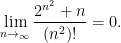
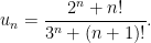
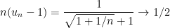
This allows us to compute many limits very easily: it is enough to identify who wins. Consider for instance the problem of finding the limit of

$\displaystyle u_n = \frac{\log^5 n + n^2}{2^n}.$

It is of the type $\infty / \infty$ . Now, informally, the hierarchy of Theorem III.1 tells us that the $\log$ is much smaller than the power of $n$ , which is itself much smaller than the geometric sequence. So the denominator should win, and the limit be 0.

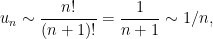
To be precise, Theorem III.1 and the properties of little o tell us that $\log^5 n = o(2^n)$ and $n^2 = o(2^n)$ , and therefore

$\displaystyle \log^5 + n^2 = o(2^n)$

and thus

$\displaystyle u_n = o(1),$

which means

$\displaystyle \lim_{n \to + \infty} u_n = 0.$

It is nice to use Theorem III.1. in conjunction with the previous properties.

Let us find the limit of

$\displaystyle \frac{2^{n^2}+n}{(n^2)!}.$

It does not fit right away as a specific case of Theorem III.1. However, we know $2^n = o(n!)$ , and we can replace $n$ by $n^2$ to obtain $2^{n^2} = o((n^2)!)$ . Similarly, $\sqrt{n} = o(n!)$ so $n = o((n^2)!)$ . Summing, we obtain $2^{n^2} + n = o((n^2)!)$ , and therefore

$\displaystyle \lim_{n \to _ \infty} \frac{2^{n^2}+n}{(n^2)!} = 0.$

Compute the limits of the following sequences as $n \to + \infty$ .

$\displaystyle \frac{\log n}{\sqrt{n}}, \quad \frac{\log \sqrt{n}}{n}, \quad \frac{n^3}{2^n}, \quad n^4 e^{-n^2}, \quad \frac{n \log n}{(n+1)^3}, \quad \frac{3^n + 4 n^5}{\sqrt{n!}}.$

Obtaining equivalents

Theorem III.1, coupled with Theorem I.2, allows to easily obtain equivalents, as follows. First, look at each sum, and only keep the largest term: this gives us an equivalent of the sum. Then multiply and divide equivalents, to find an equivalent of the final expression. Let us for instance look at

$\displaystyle u_n = \frac{2^n + n!}{3^n + (n+1)!}.$

For the numerator, we have $2^n = o(n!)$ , so $2^n + n! \sim n!$ (by Theorem I.2). Similarly, for the denominator, $3^n = o(n!) = o((n+1)!)$ , and thus $3^n + (n+1)! \sim (n+1)!$ . We therefore deduce that

$\displaystyle u_n \sim \frac{n!}{(n+1)!} = \frac{1}{n+1} \sim 1/n,$

where we use at the end that $n+1 = n + o(n)$ , so $n+1 \sim n$ .

You may want to ask your computer what it thinks of $u_{1000}$ . Probably, you will get an overflow error. Yet, this simple computation tells us that $u_{1000} \approx 0.001$ .

Asymptotic expansion

Definition

In general, we want to use little o to say: this sequence looks like this much more simple sequence, plus something which is small, where this “small” is given by a little o. This motivates the following definition.

Consider sequences $(u_n), (v_n), (w_n)$ . We write

$\displaystyle u_n = v_n + o(w_n)$

$\displaystyle u_n - v_n = o(w_n).$

Typically, $(v_n)$ and $(w_n)$ should be simple sequences (for instance made of power or geometric sequences), and $(w_n)$ should be a little o of $(v_n)$ . It makes sense to write

$\displaystyle n + o(n^3)$ 😦

but it has no relevance: $n + o(n^3) = o(n^3)$ . Take $n = 100$ . We are saying that we have 100 bucks + much less than a million. The only relevant thing is that we have much less than a million!

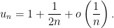
An expression of the type $u_n = v_n + o(w_n)$ , is called an asymptotic expansion of $(u_n)$ . It is telling us that $(u_n)$ is well approximated by $(v_n)$ . The accuracy of the approximation is given by the $(w_n)$ .

Let us try to find an asymptotic expansion of $u_n = \sqrt{1+1/n}$ . First, the limit of $(u_n)$ is 1, and therefore

$\displaystyle u_n = 1 + o(1).$

Now, we would like a bit more, i.e. knowing how small is $u_n - 1$ . So we write it out and use the usual trick of the conjugate quantity.

$\begin{aligned} u_n - 1 & = \sqrt{1+1/n} - 1 \\ & = \frac{(\sqrt{1+1/n}-1)(\sqrt{1+1/n} + 1)}{\sqrt{1+1/n}+1} \\ & = \frac{1/n}{\sqrt{1+1/n}+1}. \end{aligned}$

The denominator tends to 2. Therefore, we see that this should look like $1/(2n)$ . To be precise, this shows that

$\displaystyle n(u_n-1) = \frac{1}{\sqrt{1+1/n}+1} \to 1/2$

which means $n(u_n - 1) - 1/2 = o(1)$ , and thus $u_n - 1 - 1/(2n) = o(1/n)$ , which means that we have the asymptotic expansion

$\displaystyle u_n = 1 + \frac{1}{2n} + o \left ( \frac1n \right ).$

A more expeditious way is to use equivalents: by the first computation, we get

$\displaystyle u_n - 1 = \frac{1/n}{\sqrt{1+1/n}+1} \sim \frac{1}{2n},$

which means exactly, by Theorem I.2, $u_n - 1 - 1/2n = o(1/(2n)) = o(1/n).$

Algebra of little o

Example IV.1 is a bit tedious to unfold completely, but we in fact could guess the answer after the first couple lines of computation. In essence: we can do basic algebra on asymptotic expansions. We shall not write this as a formal proposition, which would be just cumbersome and incomprehensible. Working through a few examples should give us the gist of it.

Assume for instance that $u_n = n^2 + 2n - 1 + o(1/n)$ and that $v_n = 4n - 3/n + o(1/n^2)$ . We can then make computations as in basic algebra. For instance, we can compute an expansion of the sum, as follows.

$\begin{aligned} u_n + v_n & = n^2 + 2n - 1 + o(1/n) + 4n - 3/n + o(1/n^2) \\ & = n^2 + 6n - 1 - 3/n + o(1/n). \end{aligned}$

Note how the $o(1/n^2)$ of the expansion of $v_n$ disappears, or rather, is absorbed into the $o(1/n)$ . As we only know $u_n$ up to a precision of $o(1/n)$ , any extra precision on $v_n$ is irrelevant.

Similarly, we can compute a product, as follows.

$\begin{aligned} u_n v_n & = (n^2 + 2n - 1 + o(1/n)) (4n - 3/n + o(1/n^2)) \\ & = 4 n^3 - 3n + o(1) + 8 n^2 - 6 + o(1/n) - 4n + 3/n + o(1/n^2) + o(1) + o(1/n^2) + o(1/n^3) \\ & = 4 n^3 + 8n^2 - 7 n - 6 + o(1). \end{aligned}$

Similarly, anything smaller than our worse precision, here $o(1)$ , should be disregarded. With practice, we could shorten much more: namely, the second line of this computation is far too explicit. We see that the worst precision we get is $o(1)$ . Therefore, we do not need to write anything smaller. Similarly, let us try to compute an expansion of $u_n^2$ . The worst we will get is $o(n)$ . We can then disregard anything smaller, and quickly obtain

$\begin{aligned} u_n^2 & = (n^2 + 2n - 1 + o(1/n))^2 \\ & = n^4 + 4n^2 + 4 n^3 - 2 n^2 - 4n + o(n) \\ & = n^4 + 4 n^3 + 2n^2 - 4n + o(n). \end{aligned}$

Assume that $u_n = n^2 + 2 n + 3 + 4/n + o(1/n)$ and $v_n = -1/n + 2/n^2 + o(1/n^4)$ . Compute an asymptotic expansion of $u_n + v_n$ and of $u_n v_n$ .

Use Example IV.1 to compute, as efficiently as possible, an asymptotic expansion of $(1+1/n)^{3/2}$ , of the form $a + b/n + o(1/n)$ .

Expansions of power functions

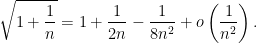
We already had plenty of fun with the asymptotic expansion

$\displaystyle \left( 1 + \frac1n \right)^{1/2} = 1 + \frac{1}{2n} + o \left ( \frac1n \right ).$

This can be generalized in two senses: either by changing the exponent, or by getting more terms in the expansion. With the techniques we introduced, getting more terms leads to more and more complicated computations. However, you can try your hand on the following.

Compute, an asymptotic expansion of $\sqrt{1+1/n}$ of the form

$\displaystyle \sqrt{1+\frac1n} = 1 + \frac{1}{2n} + \frac{a}{n^2} + o \left( \frac{1}{n^2} \right)$ ,

for some well-chosen $a$ .

Getting a first-order expansion (of the form $1 + a/n + o(1/n)$ ) of $(1+1/n)^{\alpha}$ is however doable quite generally with basic algebra.

Show that, for any $q \in \mathbb{N}$ , $q \neq 0$ , we have
$\displaystyle \left( 1 + \frac1n \right)^{1/q} = 1 + \frac{1}{qn} + o \left ( \frac1n \right ).$

You may want to remember that

$\displaystyle x - y = (x^{1/q} - y^{1/q})(x^{(q-1)/q} + x^{(q-2)/q} y + \cdots + y^{(q-1)/q}).$
Conclude that for any $p, q \in \mathbb{N}$ , $q \neq 0$ ,
$\displaystyle \left( 1 + \frac1n \right)^{p/q} = 1 + \frac{p}{qn} + o \left ( \frac1n \right ).$
Compute
$\displaystyle \lim_{n \to + \infty} n^2 \left [ 2 \left ( 1 + \frac{1}{n^2} \right )^{2/3} - \sqrt{4 + \frac{1}{n}} + \frac{1}{2n} \right ].$

Derivatives and little o

Similarly to equivalents, we can use derivatives to obtain new asymptotic expansions. As before, this relies on the fact that, when $x$ is close to $x_0$ ,

$\displaystyle f(x) - f(x_0) \approx (x - x_0) f'(x_0).$

Replacing $x$ by a sequence converging to 0 exactly yields the following result.

Assume that $f$ is differentiable at $x_0 \in \mathbb{R}$ , and that $(u_n)$ is a sequence converging to $x_0$ . Then we have the asymptotic expansion

$\displaystyle f(u_n) = f(x_0) + (u_n-x_0) f'(x_0) + o(u_n-x_0).$

Note how the right-hand side of $f(u_n) = f(x_0) + (u_n-x_0) f'(x_0) + o(u_n-x_0)$ is much simpler than $f(u_n)$ . Note also that, unlike equivalents, we do not need to assume $f'(x_0) \neq 0$ ; in this case, our expansion is just a constant (maybe $0$ as well), and a little o.

Again, the proof of this fact is essentially the definition of the derivative.

Show Theorem IV.2.

In most of the cases, we will have $x_0 = 0$ , and $f$ is a usual function, from which we can deduce the following.

If $u_n \to 0$ , then we have the following asymptotic expansions.

$e^{u_n} = 1 + u_n + o(u_n)$ .
$\log(1+u_n) = u_n + o(u_n)$ .
$\sin(u_n) = u_n + o(u_n)$ .
For any $\alpha \in \mathbb{R}$ , $(1+u_n)^{\alpha} = 1 + \alpha \: u_n + o(u_n).$

We may want to notice that the last expansion gives another much more simple approach to Exercise IV.4. Arguably, it however does not provide the insight that Exercise IV.4 provides.

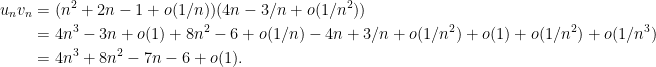
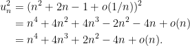
Now, this result allows us to do computations as follows. We have

$\begin{aligned} \cos \left( \frac1n \right) - \sqrt{1+\frac1n} & = 1 + o \left ( \frac1n \right ) - \left [ 1 + \frac{1}{2n} + o \left ( \frac1n \right ) \right ] \\ & = - \frac{1}{2n} + o \left ( \frac1n \right ). \end{aligned}$

From this asymptotic expansion, we deduce for instance that

$\displaystyle \lim_{n \to +\infty} n \left( \cos \left( \frac1n \right) - \sqrt{1+\frac1n} \right) = - \frac12$ .

Consider

$\displaystyle u_n = n(\log(1+2/n^2) - 2 \sin^2(1/n))$ .

We can compute

$\begin{aligned} u_n & = n \left [ \frac{2}{n^2} + o \left ( \frac{1}{n^2} \right ) - 2 \left( \frac{1}{n} + o \left ( \frac{1}{n} \right ) \right)^2 \right ] \\ & = n \left [ \frac{2}{n^2} + o \left ( \frac{1}{n^2} \right ) - 2 \left( \frac{1}{n^2} + o \left ( \frac{1}{n^2} \right ) \right) \right ] \\ & = n \left [ o \left ( \frac{1}{n^2} \right ) \right ] \\ & = o \left ( \frac1n \right ).\\ \end{aligned}$

In particular, $(u_n)$ tends to 0. But we know even more: it tends to 0 at a speed much faster than $1/n$ .

Give the best asymptotic expansion that you can of

$\displaystyle u_n = (e^{1/n^2} - 1)^2 + 3 \sin^4(1/n).$

Asymptotic expansion and equivalents

Recall from Theorem I.2 that $u_n \sim v_n$ if and only if $u_n = v_n + o(v_n)$ . Remember as well that, in an equivalent, we do not write sums, but only keep the largest term. Therefore, to get an equivalent from an asymptotic expansion, we really want to reduce the expansion to $u_n = v_n + o(v_n)$ , where $v_n$ only contains one term, absorbing everything else into the little o. In other words, an expression is equivalent to the first term of its asymptotic expansion.

For instance, we showed in Exercise IV.3 (spoiler alert!) that

$\displaystyle \sqrt{1+\frac1n} = 1 + \frac{1}{2n} - \frac{1}{8n^2} + o \left( \frac{1}{n^2} \right).$

We can therefore deduce the following, in increasing order of precision.

$\sqrt{1+1/n} = 1 + o(1)$ , so $\sqrt{1+1/n} \sim 1$ , i.e. $\sqrt{1+1/n} \to 1.$
$\sqrt{1+1/n} - 1 = 1/(2n) + o(1/n)$ , so $\sqrt{1+1/n} - 1 \sim 1/(2n).$
$\sqrt{1+1/n} - 1 - 1/(2n) = -1/(8n^2) + o(1/n^2)$ , so $\sqrt{1+1/n} - 1 - 1/(2n) \sim - 1/(8n^2).$

What about ratios?

We already saw that we can divide a comparison $u_n = o(x_n)$ by some fixed quantity, but there is no way to divide little o directly. There is however a way to divide by a nontrivial asymptotic expansion, by using the fact (Theorem IV.3) that if $u_n \to 0$ , then

$\displaystyle \frac{1}{1+u_n} = 1 - u_n + o(u_n)$ .

Therefore, we are justified to do the following computation, using the fact that $\sin(1/n) \sim 1/n$ and Proposition II.2,

$\begin{aligned} \frac{1}{1 + \sin \frac1n} & = 1 - \sin \frac1n + o \left ( \sin \frac1n \right ) \\ & = 1 - \left ( \frac1n + o \left( \frac1n \right) \right) + o \left( \frac1n \right) \\ & = 1 - \frac1n + o \left( \frac1n \right). \end{aligned}$

If the denominator (say $w_n$ ) is not of the form $w_n = 1 + u_n$ where $u_n \to 0$ , we just need to make it appear! Find a simple equivalent $v_n$ of $w_n$ by keeping the largest term, and write

$\displaystyle w_n = v_n (1 + u_n),$

where $u_n \to 0$ . We know we can divide by the (fixed and simple) $v_n$ , then we can use the previous trick on $1/(1+u_n)$ , then multiply both expansions.

Consider $u_n = 4n^2 - 2n + o(1)$ and $v_n = 2n + 6 + o(1/n)$ . Then

$\begin{aligned} \frac{u_n}{v_n} & = \frac{4n^2 - 2n + o(1)}{2n + 6 + o(1/n)} \\ & = \frac{4n^2 - 2n + o(1)}{2n(1 + 3/n + o(1/n^2))} \\ & = (2n - 1 + o(1/n)) \frac{1}{1 + 3/n + o(1/n^2))} \\ & = (2n - 1 + o(1/n)) (1 - 3/n + o(1/n) + o(1/n^2)) \\ & = (2n - 1 + o(1/n)) (1 - 3/n + o(1/n)) \\ & = 2n - 6 - 1 + o(1) \\ & = 2n - 7 + o(1).\\ \end{aligned}$

Notice that we could get a better precision (to order $o(1/n)$ ), if we knew a better expansion of $1/(1+...)$ , which we do not… for now.

Find an expansion of $\tan(1/n)$ of the type $a + b/n + o(1/n)$ , without using Theorem IV.2.
If $u_n = 3 + 1/n - 1/n^2 + o(1/n^2)$ and $v_n = 1/n + 3/n^2 + o(1/n^3)$ , find the best expansion you can of $u_n/v_n$ .

Some words of caution

Keep it simple

As mentioned before, the point of an asymptotic expansion is to make things more simple. In particular, the little o part conveys the error that we make, and as such, should only be an order of magnitude.

Careful. No sum or multiplicative constants in little o.

For instance, it is the same to write $o(3 n^2)$ or $o(n^2)$ (check the definition!), so we shall of course write the latter. Similarly, it is also exactly the same to write $o(2^n + n^2)$ or $o(2^n)$ , since the geometric sequence wins over, and we shall therefore write $o(2^n)$ only.

No cancellations

In all our computations, we always kept the little o. They are meant to convey the imprecision, and imprecision always gets worse. If we have a mediocre count of the number of people $N_1$ in a classroom, and a mediocre count of a the number of people $N_2$ who leave during the lecture, we will not magically get a very accurate number $N_1 - N_2$ of the people remaining!

Careful. Little o do not cancel out.

In other words, if we do not want little o, we should never have any to begin with.

Functions of little o

Like equivalents, it is not possible to take functions of little o. In other words, if $u_n = o(v_n)$ , and $f$ is some function, then we cannot guarantee that $f(u_n) = o (f(v_n))$ 😦 Take for instance $u_n = n$ , $v_n = n^2$ , and $f = \log$ .

Careful. It is wrong to take functions of little o.

It would be a good idea to compare this with Theorem II.8!

Extra exercises

For $p \in \mathbb{N}$ and $u_n \to 0$ , find an asymptotic expansion of $(1+u_n)^p$ of the form
$\displaystyle (1+u_n)^p = 1 + p \: u_n + q \: u_n^2 + o(u_n^2),$

for some well-chosen $q$ .
Compute

$\displaystyle \lim_{n \to + \infty} n \left ( \sqrt{1 + \frac{6}{\sqrt{n}}} - \left ( 1 + \frac{1}{\sqrt{n}} \right )^3 \right ).$

Compute the limits of the following sequences as $n \to + \infty$ , using equivalents, little o, both, or neither.

$\displaystyle \frac{\log^2 n}{\sqrt{n}}, \quad \frac{\log (n^2)}{n}, \quad n \tan(1/n), \quad 2^n e^{-n^2}, \quad n \log(1/n),$

$\displaystyle \frac{n \: 3^{1/n}}{3^{1/n} - 1}, \quad (\tan(2/n))^n, \quad (e^n + 1)^{1/n}, \quad \frac{(n!)^n}{n^{4n}}, \quad \frac{(n^2 - n)^{1/3} - n}{\log(1+\sin(1/n))},$

$\displaystyle n \log \left ( \frac{5^n + (n+1)!}{n^4 + n (n!)} \right ), \quad (2n+1) \log \left( \frac{2n-3}{2n+5} \right), \quad n^n \left ( \sin \left ( \frac{1}{2n} \right) \right )^n.$

Asymptotic comparison – II

Formal definition

Properties

Basic comparisons

Transitivity

Simplification

Multiplication

Sum

Division

Constants

Equivalents and limits

Change of time

Classical comparisons

Comparative growth

Obtaining equivalents

Asymptotic expansion

Definition

Algebra of little o

Expansions of power functions

Derivatives and little o

Asymptotic expansion and equivalents

What about ratios?

Some words of caution

Keep it simple

No cancellations

Functions of little o

Extra exercises

Published by Raoul Normand

Leave a Reply Cancel reply

Formal definition

Properties

Basic comparisons

Transitivity

Simplification

Multiplication

Sum

Division

Constants

Equivalents and limits

Change of time

Classical comparisons

Comparative growth

Obtaining equivalents

Asymptotic expansion

Definition

Algebra of little o

Expansions of power functions

Derivatives and little o

Asymptotic expansion and equivalents

What about ratios?

Some words of caution

Keep it simple

No cancellations

Functions of little o

Extra exercises

Like this:

Published by Raoul Normand

Leave a Reply Cancel reply